Explanation of the Outputs
Brief description of the procedure
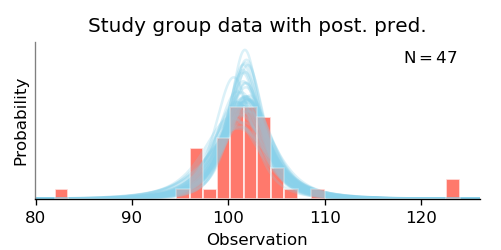
BEST models the data as samples from a t-distribution, which is a distribution much like the Gaussian (normal) distribution, with an additional parameter that controls the prevalence of outliers. After assigning a prior distribution to the parameters, these distributions are updated in accordance with how well each parameter setting fits the data, resulting in the so-called posterior distribution. (The model used by this library is not exactly like the one described in (Kruschke, 2013); the Model history page gives an exact description.)
The resulting t-distributions can be plotted with the plot_data_and_prediction() function,
whose output is a figure like this:
Variables
A BestResults object contains posterior samples of every variable of the model –
meaning .
Most of the variables are plotted by plot_all(),
but any variable can be plotted separately with plot_posterior().
The posterior samples of a given variable (e.g., Mean) can be extracted from a BestResults object (called best_out) as best_out.trace['Mean'].
The result of a one-group analysis (i.e., a BestResultsOne object) has samples of the following variables:
Mean: mean of the t-distribution that models the data. Denoted as μ.Sigma: scale parameter of the t-distribution that models the data. Denoted as σ.Normality: “normality” parameter of the t-distribution. For details, see below. Denoted as ν.SD: standard deviation of the t-distribution. Equal to \(\sigma \sqrt{\nu / (\nu - 2)}\). Often denoted as “sd”.Effect size: the difference between the mean and the given reference value, relative to the standard deviation. For each credible combination of means and standard deviations, the effect size is calculated as \((\mu - \mathrm{ref\_val}) / \mathrm{sd}\).
Some undocumented variables, such as Log sigma,
are used only as a means to an end (in this case, to calculate Sigma).
The result of a two-group analysis (i.e., a BestResultsTwo object) has samples of the following variables:
Group 1 mean: mean of the t-distribution that models group 1. Denoted as \(\mu_1\).Group 1 sigma: \(\sigma\) parameter of the t-distribution that models group 1. Denoted as \(\sigma_1\).Group 1 SD: standard deviation of the model of group 1. Denoted as \(\mathrm{sd}_1\).Group 2 mean: mean of the t-distribution that models group 2. Denoted as \(\mu_2\).Group 2 sigma: \(\sigma\) parameter of the t-distribution that models group 2. Denoted as \(\sigma_2\).Group 2 SD: standard deviation of the model of group 2. Denoted as \(\mathrm{sd}_2\).Normality: “normality” parameter of the t-distributions of both groups. For details, see below. Denoted as \(\nu\).Difference of means: the difference of the means of the two groups. Calculated as \(\mu_1 - \mu_2\).Difference of SDs: the difference of the standard deviations of the two groups. Calculated as \(\mathrm{sd}_1 - \mathrm{sd}_2\).Effect size: difference of the means, relative to the average standard deviation of the groups. For each credible combination of means and standard deviations, the effect size is calculated as \((\mu_1 - \mu_2) \,\big/\, \sqrt{(\mathrm{sd}_1^2 + \mathrm{sd}_2^2) \,/\, 2}\).
Normality
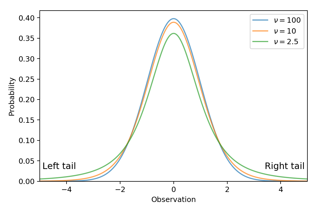
The normality parameter of Student’s t-distribution (denoted by the Greek letter nu, \(\nu\)) controls the likelihood of strong outliers: the larger this parameter, the more centered the distribution, meaning data points far from the mean are less likely. We refer to this parameter as “normality” – instead of the conventional “degrees of freedom” [1] – because a \(t_\nu(\mu, \sigma)\) distribution approximates a \(\mathrm{Normal}(\mu, \sigma)\) distribution increasingly better as \(\nu\) increases. The below figure plots t-distributions with different normality parameters, with the important difference in the tails of the distributions:
The Normality plot produced by plot_all() shows credible values of the
normality parameter in the t-distribution.
The values are shown on a logarithmic scale, because the shape of the t-distribution changes
noticeably for values of \(\nu\) near 3 but changes relatively little for \(\nu > 30\).
If the Normality histogram shows that most of the likely values of \(\nu\) are relatively low (below ~10),
then the credible t-distributions are heavy-tailed to accommodate outliers in the data;
if \(\nu\) is large (above ~30), the distributions of the groups are nearly normal.
Plots: mean vs. mode
The current implementation shows the mean of the posterior samples for distributions that are usually symmetric (such as the mean of a group), and the mode used for distributions that are usually skewed (such as the standard deviation), in accordance with the original publication (Kruschke, 2013). This behavior may change in the future.
In any case, it is advised to note the HPD interval together with the mean or the mode.
Footnotes
| [1] | Whereas the “degrees of freedom” name arises from how the t-distribution is commonly used, which is not intrinsic to the distribution. |